Convergence Against Expectations

An Exciting but Ultimately Rather Disappointing Investment

Consider a hypothetical investment whose expected¹ rate of return is 12.5% per day, independently across days. Over a year, the expected rate of return is an astronomical $4\times {10}^{20}$ percent gain. So if you invest all of your savings for a year, your expected payoff is roughly equal to the number of grains of sand on earth. Would you invest?

Would you be surprised to learn that the very same investment can also have a 97% chance of losing money over the year, and will tend to lose more money the longer you invest — and can be guaranteed to eventually lose any amount of money you put in?

In this post, I’ll use a simple toy model to show how this strange phenomenon, which I’ll call convergence against expectations, really can happen — no tricks, no verbal sleight-of-hand. My aim is to explore how we can have two intuitions, seemingly at odds with each other, but both well-founded, about how a stochastic process such as an investment will evolve over time. These dueling intuitions will be reconciled using basic probability theory and simple graphs, as all combatants ought to be.

But when we think about what, exactly, one should do about this investment, we find once again that multiple answers are reasonable.

Along the way, we will see how an expected value, as defined in statistics, can diverge wildly from the values that are most probable. Consequently, one must sometimes choose between predictions that are unbiased, and predictions that are asymptotically consistent. For those of us in fields where both unbiasedness and consistency are considered nearly sacrosanct and usually coincide asymptotically, this dilemma encourages a form of heresy, one that leads down the crooked road to Bayesian decision theory.

However, along this road, some of the graphs are pretty…

Setup: No tricks

We’ll use a standard toy model of a financial asset that evolves multiplicatively. Suppose the initial dollar value of the investment is some fixed, arbitrary $S_0>0$. Let the dollar value on integer day $T>0$ be

$$S_T=S_0\cdot R_1\cdot R_2\cdot \cdots \cdot R_T$$

where we interpret each $R_t>0$ as the proportional change in dollar value on day $t$. For all $t=1,2,\dots$, let $R_t$ be independent and identically distributed random variables that take the values $7/4$ or $1/2$ with equal probability. That is, $Pr(R_t=7/4)=Pr(R_t=1/2)=1/2$.

That’s it for our assumptions; nothing up my sleeves. Now we can start verifying some of my absurd claims.

Exponential Increase? Yes.

The expected proportional change in dollar value on any day $t$ is $\mathbb{E}[R_t]=1/2\cdot 7/4+1/2\cdot 1/2=1.125$, or a 12.5% return, as promised.

For independent random variables, the expectation of the product is simply the product of the expectations:

$$\mathbb{E}[S_0{R}_1\cdot \cdots \cdot R_T]=S_0\mathbb{E}[R_1]\cdot \cdots \cdot \mathbb{E}[R_T]=S_0(1.125{)}^T$$

So we see that the expected value of $S_T$ increases exponentially with $T$, becoming astronomically large when $T=365$, as promised. More formally, we can say that $S_0(1.125{)}^T$ is an unbiased predictor of $S_T$, meaning that the (trivial) expected value of $S_0(1.125{)}^T$ equals the expected value of $S_T$.

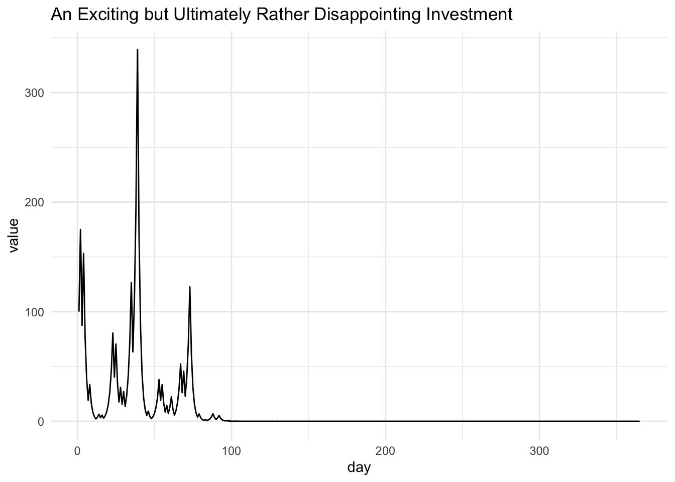
It sounds splendid to be unbiased, and even more splendid to expect exponential growth, so let’s drop the math, quit our jobs, throw in 100 dollars and watch how filthy rich we get in a year:

Given that our expectation — our unbiased prediction — was exponential growth, this piddling outcome looks like a computer glitch or a math error. But it’s not. The final value of our $100 investment really is essentially zero, and this is representative of most draws from the stochastic process we have described. But the expected value really is exponentially increasing. What in the name of Pierre-Simon Laplace is going on?

Exponential Decrease? Yes.

In the previous section, we answered the following question:

1. How much money do you expect to have gained from this investment in a year?

However, we could have posed a very similar but not identical question:

2. How much do you expect to have gained money from this investment in a year?

The first question was about $\mathbb{E}[S_T-S_0]$. The second is about $Pr(S_T>S_0)$. They have very different answers.

Consider: for any $S_T$, the expected number of increases (where $R_t=7/4$) equals the number of decreases (where $R_t=1/2$); and if the numbers of increases and decreases are equal, well, $7/4\cdot 1/2=7/8$, which is less than one, so there is still a net decrease in value. This, ultimately, is what dooms our investment.

We can quantify this net decrease more precisely. To start, let’s make a new variable $Y_T=\frac{1}{T}\ln S_T$ that converts $S_T$ into a sample average, which is easier to work with:

$$Y_T=\frac{1}{T}\ln S_0+\frac{1}{T}\sum _{t=1}^T\ln R_t$$

Applying our good friend Chebyshev’s Inequality,² we have an expression that bounds $Y_T$ in probability. For any distance $\delta >0$,

$$Pr(|Y_T-{\mu }_T|>\delta )\le \frac{{\sigma }_T^2}{{\delta }^2}$$

where ${\mu }_T:=\mathbb{E}[Y_T]=\frac{1}{T}\ln S_0+\mathbb{E}\ln R$ (we drop the subscript of $R_t$ because they’re iid), and ${\sigma }_T^2:=\mathbb{V}(Y_T)=\mathbb{V}(\frac{1}{T}\sum _{t=1}^T\ln R)=\frac{1}{T}\mathbb{V}(\ln R)$. Note that as $T$ increases, ${\mu }_T⟶\mathbb{E}[\ln R]\approx -0.07$ and so for large enough $T$, we have ${\mu }_T<0$.

Taking the complement in probability and substituting ${\sigma }_T^2:=\mathbb{V}(Y_T)=\frac{1}{T}\mathbb{V}(\ln R)$,

$$\begin{array}{rl}Pr(-\delta & \le Y_T-{\mu }_T\le \delta )\ge 1-\frac{\mathbb{V}(\ln R)}{T{\delta }^2}\end{array}$$ Substituting in the definition of $Y_T$ and rearranging, we conclude:

$$\begin{array}{rl}Pr(\exp \{T({\mu }_T-\delta )\}& \le S_T\le \exp \{T({\mu }_T+\delta )\})\ge 1-\frac{\mathbb{V}(\ln R)}{T{\delta }^2}\end{array}$$

This expression says that as $T$ increases, $S_T$ has an increasing probability $1-\frac{\mathbb{V}(\ln R)}{T{\delta }^2}$ of being bounded between two exponential functions which converge to zero.³

We have established that as $T$ increases, $S_T$ converges in probability to 0. Using the Strong Law of Large Numbers⁴, we could also prove a related fact: $S_T$ converges almost surely (that is, with probability one) to zero. So in the limit all money is lost, with probability one.

Hmmmmmm. Earlier we found that as $T$ increases, the expected value of $S_T$ increases exponentially. But now we find that $S_T$ decreases to zero exponentially quickly…

Reconciling our intuitions: Convergence against Expectations

The question, mathematically, is how to have the expectation $\mathbb{E}{S}_T$ increase exponentially, even while $S_T$ has a high probability of decreasing exponentially.

There’s only one way: the sequence $(S_T)$ must tend to contain large but improbable “excursions” in the positive direction. As $T$ increases, these excursions must become increasingly large — pulling the average up — but also increasingly improbable — pulling the limit down.

To visualize this, we can run 10,000 simulations of trajectories starting at $1, from $t=1$ to $t=100$, and plot them, along with the daily 99% quantile (in red) for reference.

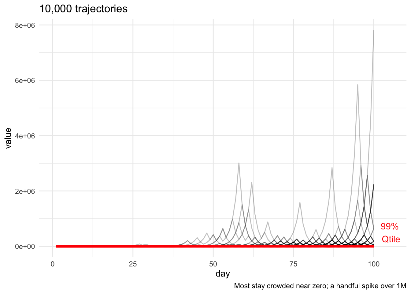
So, on any given day, 99% of trajectories are below the red line, which is far, far below the highest trajectories, a handful of which spike into the millions — pulling up the average.

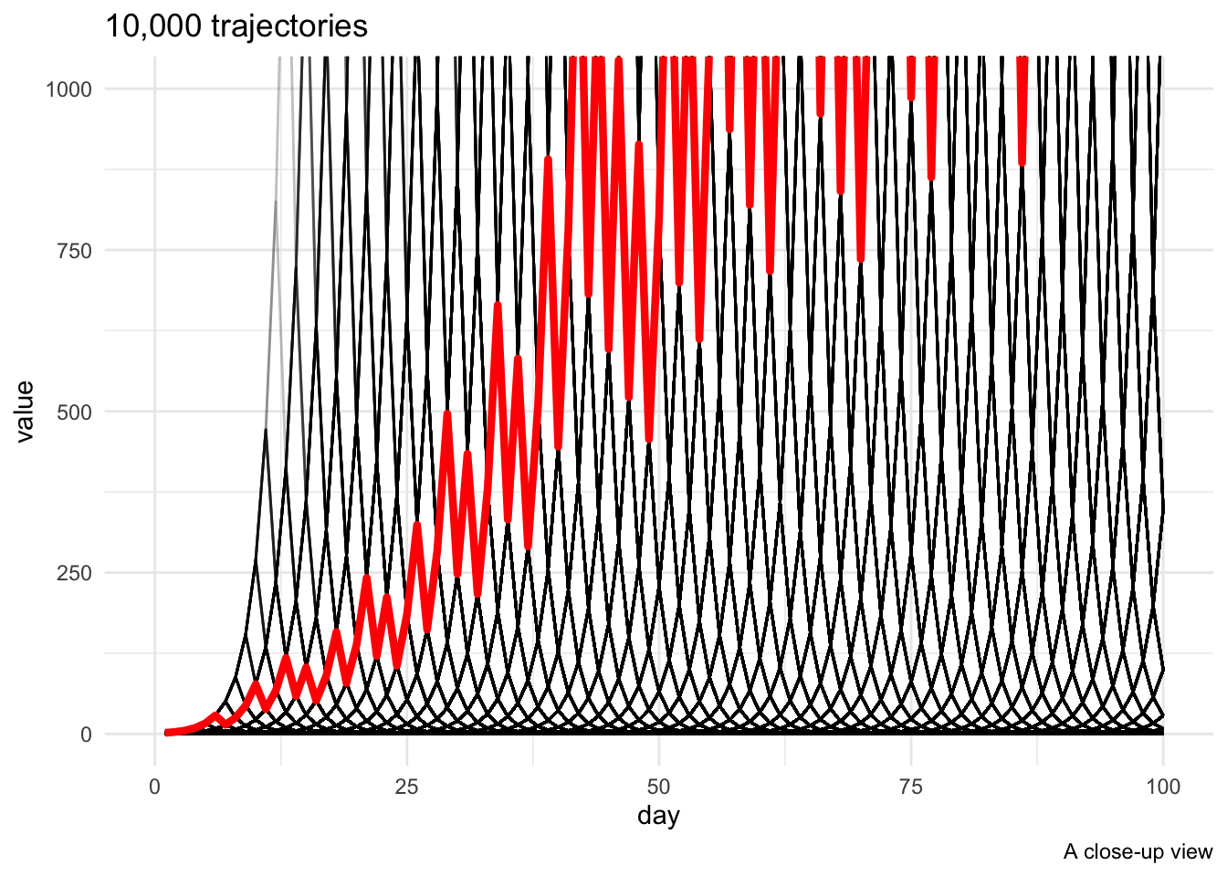
Zooming in, we see a pretty latticework of transient exponential increases and decreases; temporarily, the 99th percentile rises out of sight.

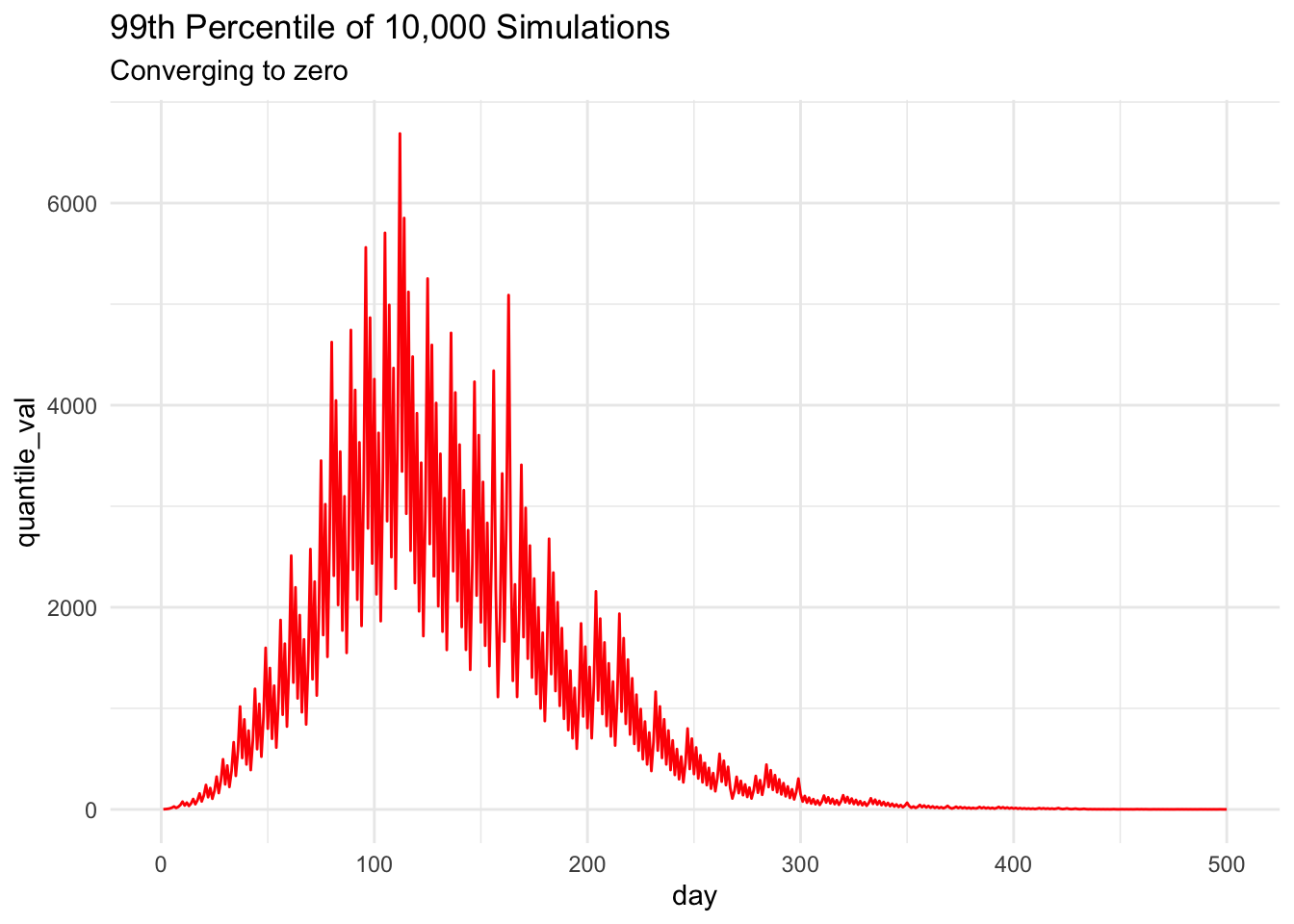
However, plotting the daily 99th percentile⁵ over a longer period, we can see that convergence to zero really does happen⁶ — eventually, after an intriguing excursion into the thousands (our proof was about limiting behavior, so it’s not contradicted by this short-run behavior). Because of our proof of convergence, we know that we could pick any percentile, however high, and eventually it would converge to zero as above.

But is it a good investment?

Mathematically, the paradox is resolved (or, for the wonderless pedants, never existed). Because $S_T$ contains excursions that are increasingly large but increasingly improbable, the expectation $\mathbb{E}{S}_T$ increases exponentially with $T$, even while $S_T$ itself becomes overwhelmingly likely to decrease exponentially. These facts are mutually consistent, even if they may conflict with our intuitions about what an expected value is.

But this resolution might still seem unsatisfying; we haven’t yet said what to do about the investment. Is it a good investment or not?

The conventional answer (which I think it’s healthy to be skeptical of) is that it depends on your preferences for risk. For large $T$, $S_T$ is essentially a gamble with a very large chance of losing nearly everything you put in, and a very small chance of doing extremely well — with a large positive expected monetary value. Whether the expected utility value of this risky gamble is positive depends on the shape of your utility function — specifically, its concavity.

If your utility function is linear in money — meaning that it has no concavity, and you have no aversion to risk — then it’s easy to verify that the expected utility-gain from the investment is positive, because the expected money-gain is positive. So, in theory, you think it’s worth some positive amount of money to take the gamble for any finite length of time $T$ — even though it will probably lose money, exponentially fast as time increases.

If your utility function is concave — meaning that you have some aversion to risk — then you may consider it worth paying money not to take the investment, depending on the degree of concavity. For example, suppose your utility function is logarithmic in money, $u(S_T)=\ln (S_T)$. Then the expected utility gain from investing $S_0$ is

$$\mathbb{E}[u(S_T)-u(S_0)]=\sum _{t=1}^T\mathbb{E}\ln R_t$$

— and as before, we noted that $\mathbb{E}\ln R_t\approx -0.07$. So we have $\mathbb{E}[u(S_T)-u(S_0)]\approx -T\cdot 0.07$: so with logarithmic utility, this investment looks increasingly bad as $T$ increases.

Personally, I’m not entirely convinced by this particular model of risk preferences, for reasons I may explore in another post. But however we model them, differences in thinking about risk or uncertainty would explain why, even after the facts are laid before us, we may disagree (even with ourselves) about whether this investment is worth taking.

Conclusion

It’s worth noting that this phenomenon isn’t a “knife-edge result” that depends on the exact numbers I use in my example; convergence against expectations will occur whenever $\mathbb{E}[R_t]>1$ while $\mathbb{E}[\ln R_t]<0$. Although for dramatic effect we discussed outlandish (for a stock market, but not for a bacterium) growth rates per day, we could always pick a time-scale that would make things seem more plausible. So I’ll end with a question that I’m still pondering: in the real world, how common are these strange phenomena that have a positive expected growth rate, but a high probability of negative growth?

Footnotes

1. In the formal sense

2. We could get tighter bounds with Hoeffding’s Inequality, but Chebyshev generalizes better, and the pursuit of maximally tight bounds is a form of masochism that I find tedious.

3. To see that the bounding functions are decreasing, note that we can always pick a $\delta$ small enough that ${\mu }_T+\delta <0$. So as $T$ increases, for small enough $\delta$ the bounds $\exp \{T({\mu }_T-\delta )\}$ and $\exp \{T({\mu }_T+\delta \}$ are both exponential functions containing $T$ with a negative coefficient — the bounding functions are decreasing to zero.

4. which applies because $\mathbb{E}{Y}_T<\mathrm{\infty }$

5. Because the sample mean depends primarily on extremely improbable events, this simple simulation doesn’t estimate it very well for large T, so I don’t plot it.

6. Technically, we can’t prove convergence by showing a simulation that seems to converge — it could always diverge again. But apparent convergence in a simulation is empirical evidence that we didn’t botch our proof.